ra.rings and algebras - Computing Integral Closures

I'm wondering if there's an algorithm, or a program I can use, to compute integral closures. Specifically, what I have in mind are variants of questions of the sort: what is the integral closure of ℤ[x] in Quot(ℚ[x,y]/fℚ[x,y]), for some specific f(x,y).

gr.group theory - Affine Weyl groups as Coxeter groups

In the abstract Bourbaki set-up, the affine Weyl group is defined to be a
semidirect product of an irreducible Weyl group with its coroot lattice.
This is naturally a Coxeter group, characterized in terms of its
positive semidefinite Coxeter matrix. The basic theory is developed
independently of applications in Lie theory, but is directly usable if you
start with a connected semisimple algebraic group (over an algebraically
closed field) and require its root system to be irreducible of type A, B,
etc. Most of the time this causes no trouble. While it is natural to work
with a connected reductive group, people often use the expression "affine
Weyl group" too loosely in this general context. For example, the standard
features of alcove geometry require irreducibility. Otherwise you have
to deal with products of simplexes, etc. In any case, the difference between
reductive and semisimple groups such as general linear and special linear
is sometimes significant.

In the Iwahori-Matsumoto (or Bruhat-Tits) setting over local fields, a
more intrinsic affine Weyl group occurs directly within the structure of
the group itself. Here one has to be cautious about applying
abstract Coxeter group theory or BN-pair theory, as I believe most authors
are. Already in the proceedings of the 1965 Boulder AMS summer institute,
Iwahori had to formulate a more complicated "generalized BN-pair" formalism
for this situation. I'm not sure what has become standard by now in the
literature.

In other situations (the classical study of compact Lie groups, or
the later application of affine Weyl groups in modular representation
theory starting with Verma) there is usually no difficulty about specializing
to the irreducible case. Here the affine Weyl group lives outside the
actual group under study. This is the situation I'm most comfortable with.

You need to make precise the setting in which you really want to study reductive groups, in order to adapt the Bourbaki language and results.
There are several distinct issues here: 1) Extra care is needed in treating
disconnected algebraic groups such as orthogonal groups, or in treating
reductive rather than semisimple groups. 2) Adjoint groups, simply
connected groups, and the occasional intermediate type: not all details of
structure are exactly the same. 3) Most important for working over
local fields is the natural use of an "extended affine Weyl group" (as in
much of Lusztig's work involving Hecke algebras, cells, etc.). Here you
start with the Bourbaki version of the affine Weyl group (a Coxeter group)
and form a semidirect product with a finite group $Omega$ isomorphic to the weight lattice mod root lattice (universal center). This amounts to
working with a semidirect product of the Weyl group and the full (co)weight
lattice rather than the (co)root lattice. Fortunately it's easy to extend
notions like length function to this extended group.

EDIT: Besides Bourbaki's treatment of Coxeter groups and root systems (1968),
foundational papers from that era include Iwahori-Matsumoto (IHES Publ. Math. 25, 1965), at http://www.numdam.org, and Iwahori's 1965 article in the AMS Boulder proceedings
http://www.ams.org/books/pspum/009/0215858/pspum0215858.pdf, followed by much more technical work by Bruhat-Tits.
Lusztig has written many technical papers on extended affine Weyl groups and corresponding affine Hecke algebras, including his four part series on cells in affine Weyl groups and later work on multiparameter cases. Much of this work is motivated by reductive groups over local fields, as well as the modular representation theory of reductive groups and their Lie algebras (where "linkage" of weights appears at first relative to an extended affine Weyl group).

mg.metric geometry - How can I embed an N-points metric space to a hypercube with low distortion?

Y. Bartal has studied a related problem of embedding metric spaces to hierarchically separated trees. With $1 < mu$ being a fixed real number, a $mu$-HST is equivalent to the set of corners of a rectangle whose edges are of length $c, cmu^{-1}, cmu^{-2}, dots, cmu^{1-D}$ with the $l_infty$-metric. That is, if you think of the space as the set of bit sequences of length $D$, the distance of two sequences is $cmu^{-j}$ if they first differ in bit $j$.

Now in your question you didn't ask for $infty$-metric, but for this set of points, it doesn't really matter which metric you take because the distortion between this and either the $l_1$ or $l_2$ metric is bounded by a constant (if you fix $mu$ but $D$ can vary).

(This metric can be considered a graph metric on a special tree, that is, one where the points are some (but not necessarily all) vertexes of a tree graph with weighted edges, and the distance is the shortest path. This is where "tree" in the name comes from.)

Now Bartal's result in [1] basically says that you can embed any metric space randomly to a $mu$-HST with distortion at most $mu(2ln n+2)(1+log_mu n)$ where $n$ is the number of points. (Also, this embedding can be computed with a randomized polynomial algorithm.)

For this, you need to know what a distortion $alpha$ random embedding $f$ means. It means that for any two points $d(x,y) < d(f(x),f(y))$ is always true and that the expected value of $d(f(x),f(y))$ is at most $alpha d(x,y)$. For many applications, this is just as good as a deterministic embedding with low distortion. In fact, you can make a deterministic embedding with low distortion from it by imagining the metric $d^* $ on the original space where $d^*(x,y) = E(d(f(x), f(y))$, but this notion isn't too useful because the resulting metric does not have nice properties anymore (it's not HST). Indeed, I believe the randomness is essential here as I seem to remember reading somewhere that you can't embed a cycle graph (with equal edge weights) to a tree graph with low distortion.

Anyway, this might not really answer your question. Firstly, $D$ (the number of dimensions of the rectangle) is not determined in advance, but that's not a real problem because if you have $D$ significantly different distances in the input metric then you need at least that large a $D$ for any embedding; and with this embedding you don't need a $D$ larger than $log_mu (Delta/delta)$ where $Delta$ and $delta$ are the largest and smallest distances in the input. The real problem is that you seem to want to know a deterministic embedding, and the highest possible distortion necessary in that case, which this really doesn't tell. For example, a cycle graph with an even number $n$ of vertexes can of course be embedded isometrically to a cube of dimension $n/2$.

Survey [2] has some more references.

[1]: Yair Bartal, On Approximating Arbitrary Metrics by Tree Metrics. Annual ACM Symposium on Foundations of Computer Science, 37 (1996), 184–193.

[2]: Piotr Indyk, Jiří Matoušek, Low-distortion embeddings of finite metric spaces. Chapter 8 in Handbook of Discrete and Computational Geometry, ed. Jacob E. Goodman and Joseph O'Rourke, CRC Press, 2004.

reference request - Are there extensive tables of Fourier transforms available online?

I hope this is suitable for MO... I was wondering if someone can suggest a website (or some online document) containing an $extensive$ table of Fourier transforms? When I try obvious Google searches, like "table of Fourier transforms", the several dozen top results give extremely short tables.

My question is in fact motivated by one concrete example (so if you know the answer to this one, please let me know!). Note that I failed to find the answer not only online, but also in the standard books with Fourier transform tables (such as "Tables of Integral Transforms" from the Bateman project). Suppose $a$ and $b$ are real numbers. The function $f(xi)=(i-xi)^acdot(log(i-xi))^b$ can be defined for all real $xi$ (by choosing appropriate branches of $log(i-xi)$ and $log(log(i-xi))$), and the inverse Fourier transform of $f(xi)$ makes sense as a distribution on $mathbb{R}$. Is there an explicit formula for it? Apparently, the answer is yes when $b$ is a nonnegative integer, but what about other values of $b$?

Ignoring this particular example, I think many people who work with Fourier transforms on a daily basis would benefit from having an easily accessible table of Fourier transforms of functions, especially ones that are quite nontrivial to compute explicitly.

$mathbf{EDIT.}$ As was commented below, the Erdelyi book "Tables of Integral Transforms" is the same as the one I referred to above when I mentioned the Bateman project. I also checked the book "Table of Integrals, Series, and Products" by Gradshteyn and Ryzhik, and couldn't find the thing I'm looking for.

co.combinatorics - Asymptotics of a Bernoulli-number-like function

[Revised and expanded to give the answer for all $k>1$ and incorporate
further terms of an asymptotic expansion as $n rightarrow infty$]

Fix $k>1$, and write $a_1=f(1,k)=1$ and
$$
a_n = f(n,k) =
frac1{1-q^{-n}} sum_{r=1}^{n-1} {n choose r} (1/k)^{n-r} (1/q)^r a_r
phantom{for}(n>1),
$$
where $q := k/(k-1)$, so $(1/k) + (1/q) = 1$. Set
$$
a_infty := frac1{k log q}.
$$
For example, if $k=2$ then $a_infty = 1 / log 4 = 0.72134752ldots$,
which $a_n$ seems to approach for large $n$, and likewise for
$k=6$ (the dice-throwing case) with $a_infty = 1/(6 log 1.2) =
0.9141358ldots$. Indeed as $n rightarrow infty$ we have
"$a_n rightarrow a_infty$ on average", in the sense that (for instance)
$sum_{n=1}^N (a_n/n) sim a_infty phantom. sum_{n=1}^N (1/n)$
as $N rightarrow infty$. But, as suggested by earlier
posted answers to Tim Chow's question, $a_n$ does not converge,
though it stays quite close to $a_infty$: we have
$$
a_n = a_infty + epsilon^{phantom.}_0(log_q n) + O(1/n)
$$
as $n rightarrow infty$, where $epsilon^{phantom.}_0$ is a smooth
function of period $1$ whose average over ${bf R} / {bf Z}$ vanishes
but is not identically zero; for large $k$ (already $k=2$ is large
enough), $epsilon^{phantom.}_0$ is a nearly perfect sine wave
with a tiny amplitude $exp(-pi^2 k + O(log k))$, namely
$$
frac2{klog q}left|phantom.Gammabigl(1 + frac{2pi i}{log q}bigr)right|
phantom.=phantom.
frac2{k log q}
left[frac{(2pi^2/ log q)}{sinh(2pi^2/ log q)}right]^{1/2}.
$$
For example, for $k=2$ the amplitude is $7.130117ldots cdot 10^{-6}$,
in accordance with numerical observation (see previously posted answers
and the plot below). For $k=6$ the amplitude is only
$8.3206735ldots cdot 10^{-23}$ so one must compute well beyond
the usual "double precision" to see the oscillations.

More precisely, there is an asymptotic expansion
$$
a_n sim a_infty + epsilon^{phantom.}_0(log_q n)
+ n^{-1} epsilon^{phantom.}_1(log_q n)
+ n^{-2} epsilon^{phantom.}_2(log_q n)
+ n^{-3} epsilon^{phantom.}_3(log_q n)
+ cdots,
$$
where each $epsilon^{phantom.}_j$ is smooth function of period $1$
whose average over ${bf R} / {bf Z}$ vanishes, and
— while the series need not converge —
truncating it before the term $n^{-j} epsilon^{phantom.}_j(log_q n)$
yields an approximation good to within $O(n^{-j})$. The first few
$epsilon^{phantom.}_j$ still have exponentially small amplitudes,
but larger that of $epsilon^{phantom.}_0$ by a factor
$sim C_j k^{2j}$ for some $C_j > 0$; for instance, the amplitude of
$epsilon^{phantom.}_1$ exceeds that of $epsilon^{phantom.}_0$
by about $2(pi / log q)^2 sim 2 pi^2 k^2$. So $a_n$ must be
computed up to a somewhat large multiple of $k^2$ before it becomes
experimentally plausible that the residual oscillation $a_n - a_infty$
won't tend to zero in the limit as $n rightarrow infty$.

Here's a plot that shows $a_n$ for $k=2$ (so also $q=2$) and
$2^6 leq n leq 2^{13}$, and compares with the periodic approximation
$a_infty + epsilon^{phantom.}_0(log_q n)$ and the refined approximation
$a_infty + sum_{j=0}^2 n^{-j} epsilon^{phantom.}_j(log_q n)$.
(See http://math.harvard.edu/~elkies/mo11255+.pdf for
the original PDF plot, which can be "zoomed in" to view details.) The
horizontal coordinate is $log_2 n$; the vertical coordinate is centered at
$a_infty = 1/(2 log 2)$, showing also the lines $a_infty pm 2|a_1|$;
black cross-hairs, eventually merging visually into a continuous curve,
show the numerical values of $a_n$; and the red and green contours
show the smooth approximations.

To obtain this asymptotic expansion, we start by generalizing
R.Barton's formula from $k=2$ to arbitrary $k>1$:
$$
a_n = frac1k sum_{r=0}^infty phantom. n q^{-r} (1-q^{-r})^{n-1}.
$$
[The proof is the same, but note the exponent $n$ has been corrected
to $n-1$ since we want $n-1$ players eliminated at the $r$-th step,
not all $n$; this does not affect the limiting behavior
$a_infty+epsilon^{phantom.}_0(log_q n)$, but is needed to get
$epsilon^{phantom.}_m$ right for $m>1$.] We would like to approximate
the sum by an integral, which can be evaluated by the change of variable
$q^{-r} = z$:
$$
frac1k int_{r=0}^infty phantom. n q^{-r} (1-q^{-r})^{n-1}
= frac1{k log q} int_0^1 phantom. n (1-z)^{n-1} dz
= left[-a_infty(1-z)^nright]_{z=0}^1 = a_infty.
$$
But it takes some effort to get at the error in this approximation.

We start by comparing $(1-q^{-r})^{n-1}$ with $exp(-nq^{-r})$:
$$
begin{eqnarray}
(1-q^{-r})^{n-1}
&=&
exp(-nq^{-r}) cdot exp phantom. [nq^{-r} + (n-1) log(1-q^{-r})]
cr
&=&
exp(-nq^{-r}) cdot
exp left[q^{-r} - (n-1) left(
frac{q^{-2r}}2 + frac{q^{-3r}}3 + frac{q^{-4r}}4 + cdots
right)
right].
end{eqnarray}
$$
The next two steps require justification (as R.Barton noted for
the corresponding steps at the end of his analysis), but the
justification should be straightforward. Expand the second factor
in powers of $u := nq^{-r}$, and collect like powers of $n$, obtaining
$$
exp(-nq^{-r}) cdot left(
1 - frac{u^2-2u}{2n} + frac{3u^4-20u^3+24u^2}{24n^2}
- frac{u^6-14u^5+52u^4-48u^3}{48n^3} + - cdots right).
$$
Each term $n^{-j} epsilon_j(log_q(n))$ ($j=0,1,2,3,ldots$)
will arise from the $n^{-j}$ term in this expansion.

We start with the main term, for $j=0$,
which is the only one that does not decay with $n$. Define
$$
varphi_0(x) := q^x exp(-q^x),
$$
which as Reid observed decays rapidly both as $x rightarrow infty$
and as $x rightarrow -infty$. Our zeroth-order approximation to $a_n$ is
$$
frac1k sum_{r=0}^infty phantom. varphi_0(log_q(n)-r),
$$
which as $n rightarrow infty$ rapidly nears
$$
frac1k sum_{r=-infty}^infty varphi_0(log_q(n)-r).
$$
For $k=q=2$, this is equivalent with Reid's formula for $R(n)$,
even though he wrote it in terms of the fractional part of $log_2(n)$,
because the sum is clearly invariant under translation of $log_q(n)$
by integers.

We next apply Poisson summation. Since
$sum_{r in {bf Z}} phantom. varphi_0(t+r)$
is a smooth ${bf Z}$-periodic function of $t$, it has a Fourier expansion
$$
sum_{min{bf Z}} phantom. c_m e^{2pi i m t}
$$
where
$$
c_m = int_0^1 left[ sum_{r in {bf Z}} phantom. varphi_0(t+r) right]
phantom. e^{-2pi i m t} dt
= int_{-infty}^infty varphi_0(t) phantom. e^{-2pi i m t} dt
= hatvarphi_0(-m).
$$
Changing the variable of integration from $t$ to $q^t$ lets us recognize the
Fourier transform $hatvarphi$ as $1/log(q)$ times a Gamma integral:
$$
hatvarphi_0(y)
= frac1{log q} GammaBigl(1 + frac{2 pi i y} {log q}Bigr).
$$
This gives us the coefficients $a_m$ in closed form. The constant coefficient
$a_0 = 1 / (log q)$ can again be interpreted as the approximation of the
Riemann sum $sum_{r in {bf Z}} phantom. varphi_0(t+r)$ by an integral;
the oscillating terms $a_m e^{2pi i m t}$ for $m neq 0$
are the corrections to this approximation, and are small due to the
exponential decay of the Gamma function on vertical strips — indeed
we can compute the magnitude $|a_m|$ in elementary closed form using the formula
$|Gamma(1+itau)| = (pitau / sinh(pitau))^{1/2}$. So we have
$$
frac1k sum_{r in bf Z} phantom. varphi_0(log_q(n)-r)
= frac1k sum_{m in bf Z} phantom. hatvarphi_0(-m) e^{2pi i log_q(n)}
= a_infty + epsilon_0(log_q(n))
$$
where $a_infty = a_0 / k = 1 / (k log q)$ as above, and
$epsilon^{phantom.}_0$, defined by
$$
epsilon^{phantom.}_0(t) =
left[ sum_{rinbf Z} phantom. varphi_0(t+r) right] - a_infty,
$$
has the Fourier series
$$
epsilon^{phantom.}_0(t)
= frac1k sum_{m neq 0} hatvarphi_0(-m) e^{2pi i m t}.
$$
Taking $m = pm 1$ recovers the amplitude $2|a_1|/k$ exhibited above;
the $m = pm 2$ and further terms yield faster but tinier oscillations,
e.g. for $k=2$ the $m=pm 2$ terms oscillate twice as fast but with
amplitude only $6.6033857ldots cdot 10^{-12}$.

The functions $epsilon^{phantom.}_j$ appearing in the further terms
$n^{-j} epsilon^{phantom.}_j(log_q(n))$
of the asymptotic expansion of $a_n$ are defined similarly by
$$
epsilon^{phantom.}_j(t) =
frac1k sum_{rinbf Z} phantom. varphi_j(t+r),
$$
where
$$
varphi_j(x) = P_j(q^x) varphi_0(x) = P_j(q^x) q^x exp(-q^x)
$$
and $P_j$ is the coefficient of $n^{-j}$ in our power series
$$
(1-q^r)^{n-1} = exp(-nq^{-r}) phantom.
sum_{j=0}^infty frac{P_j(nq^{-r})}{n^j}.
$$
Thus
$
P_0(u)=1, phantom+
P_1(u) = -(u^2-2u)/2, phantom+
P_2(u) = (3u^4-20u^3+24u^2)/24
$, etc.
Again we apply Poisson to expand $epsilon^{phantom.}_j(log_q(n))$
in a Fourier series:
$$
epsilon^{phantom.}_j(t)
= frac1k sum_{m in bf Z} hatvarphi_j(-m) e^{2pi i m t},
$$
and evaluate the Fourier transform $hatvarphi_j$ by integrating
with respect to $q^t$. This yields a linear combination of Gamma
integrals evaluated at $1 + (2pi i y / log q) + j'$ for
integers $j' in [j,2j]$, giving $hatvarphi_j$ as a
degree-$2j$ polynomial multiple of $hatvarphi_0$. The first case is
$$
begin{eqnarray*}
hatvarphi_1(y)
&=& frac1{log q} left[
GammaBigl(2 + frac{2 pi i y} {log q}Bigr)
- frac12 GammaBigl(3 + frac{2 pi i y} {log q}Bigr)
right]
\
&=& frac1{log q} frac{pi y}{log q} left(frac{2 pi y}{log q} - iright)
phantom.
GammaBigl(1 + frac{2 pi i y} {log q}Bigr)
\
&=& frac{pi y}{log q} left(frac{2 pi y}{log q} - iright)
phantom. hatvarphi_0(y).
end{eqnarray*}
$$
Note that $varphi_1(0) = 0$, so the constant coefficient of the
Fourier series for $epsilon^{phantom.}_1(t)$ vanishes;
this is indeed true of $epsilon^{phantom.}_j(t)$ for each $j>0$,
because $hatvarphi_j(0) = int_{-infty}^infty phi_j(x) phantom. dx$
is the $n^{-j}$ coefficient of a power series in $n^{-1}$ that we've
already identified with the constant $a_infty$. Hence (as can also
be seen in the plot above) none of the decaying corrections
$n^{-j} epsilon^{phantom.}_j(log_q n)$ biases the average of $a_n$
away from $a_infty$, even when $n$ is small enough that
those corrections are a substantial fraction of the
residual oscillation $epsilon_0(log_q n)$. This leaves
$hatvarphi_j(mp1) e^{pm 2 pi i t} / k$ as the leading terms
in the expansion of each $epsilon^{phantom.}_j(t)$, so we see as promised
that $epsilon^{phantom.}_j$ is still exponentially small but with
an extra factor whose leading term is a multiple of $(2pi / log q)^{2j}$.

planetary formation - How large (that is, radius) could a planet be?

Puffy planets tend to be Jupiter or Saturn like, probably lower mass than Jupiter, perhaps lower metalicity but the most important factor is heat. Either close to the sun or recently formed. Heat expands gas planets. You're correct that as you add more mass the planet of Jupiter mass tends not to grow larger, but if there's enough internal heat, gas giant planets can get a bit larger than Jupiter. Planets as much as 2 Jupiter Radii have been observed (though there's some inaccuracy in those estimates), but growing larger than Jupiter is largely a factor of high temperature.

Rocky worlds will never grow as large as Jupiter. The greater mass will prevent it, and past a certain mass, a rocky world is unlikely to remain what we consider rocky. Above a certain mass it holds onto hydrogen which is the most abundant gas in the universe, and that would give the massive rocky world an appearance more like a gas giant.

But to answer your question in theory, if you had a rocky world with Jupiter mass and a negligible atmosphere, it could never get close to Jupiter diameter. The mass crushes the inside of the planet. Mercury for example is made of denser material than the earth. Higher Iron content, but it's less dense than the Earth because the Earth's mass crushes its rocky mantle and metallic core. When you start to get a Jupiter-mass rocky world, the crushing becomes significant and you could never build a rocky world close to as big as Jupiter. As with hydrogen, it would reach a certain maximum size, then it would begin to get smaller under the crush of gravity. Even so called "non compactible" material, does compact at the pressure inside large planets. Iron has a density of 7.874 g/cm³ and slightly less than that at high temperature, but the Earth's metallic core has a density of 12.6–13.0, and that's primarily due to crushing. When you've reached Jupiter mass, the crushing and density is significantly greater.

At about the mass of the sun the planet would be smaller than the Earth, and it would basically resemble a white dwarf star, and no longer be distinguishable as a rocky world.

I can add a few links to back this up if needed and if someone wants to run the math or give an answer with more detail, feel free.

gravity - Can asteroids contain atmosphere?

At a certain size, huge asteroids get classified as dwarf planets. Pluto has an atmosphere 100,000 times thinner than Earth, and Pluto is already one of the two largest dwarf planets known.

Asteroids (like everything) do have gravity, so nearby gas would be drawn to them. But it would take just very tiny distrubances for that gas to drift away, so what little there is would probably be close to undetectable.

na.numerical analysis - Random, Linear, Homogeneous Difference Equations and Time Integration Methods for ODEs

Most methods (that I know of) of numerically approximating the solution of ODEs are "general linear methods". For this type of method, the so-called 'linear stability' is examined by applying the method to the linear, constant-coefficient, (complex) scalar ODE

$dot{y} = lambda y $.

Because the same procedure is used to generate a new approximation at each time step, the methods result in linear, homogeneous, constant-coefficient difference equations for the approximate solution values at each time step. As a result, linear stability analysis for these methods amounts to analyzing the solutions of constant coefficient, homogeneous linear difference equations.

If you vary the method randomly at each time step, the coefficients of the difference equation are no longer constant. For example, second order explicit linear multistep methods can be written as a one-parameter family. If you choose this parameter randomly at each time step, the difference equation looks like this

$y_{n+1} + F(a(n))y_n + G(a(n))y_{n-1} = 0$

where $a(n)$ is a random variable (the parameter in the family of methods) and the functions $F$ and $G$ are known. My main question is whether there is any theory giving conditions on $F$, $G$, and the distribution of $a$ such that solutions remain bounded in the limit of large $n$. It would be nice if the theory generalized to higher order difference equations too.

If you were to randomly decide to use second-order multistep versus second-order Runge-Kutta methods, for example, then $F$ and $G$ would also depend on $n$. A theory to handle that case would be welcome too.

Since the numerical analyst is free to choose the distribution of $a$, and to some extent also $F$ and $G$, I'm wondering if it might be possible to design 'random' methods that have better linear stability properties than the usual ones which repeat the same process over and over. I'm posting here because I know almost nothing about stochastic/random processes.

planet - Planetary reference systems and time

I am researching into how coordinate systems of solar systems objects are created by reading some of the reports written by the Working Group on Cartographic Coordinates and Rotational Elements (e.g. 2009). However, I am finding it difficult to completley understand the role of time in defining reference systems.

When observing at a planet from Earth, for example Jupiter, there are a variety of factors that make it difficult to construct a reference system (including no solid surface and planetary precession), so we use geometry to define a reference system. However, because our perspective is dynamic, meaning Jupiter's surface changes and the planet's move, we say that at time J2000 we know the precise orientation and position of Earth and therefore can say from position defined at J2000 this is the coordinate reference system for Jupiter.

So, does incorporating time (e.g. J2000) mean we can say a coordinate reference system is based on the situation of an object, Jupiter in this example, at a given moment?

magnetic field - Formation of a magnetosphere for gas giants / small stars

This question got me thinking about this.

Jupiter has, and presumably super-Jupiters can have a strong magnetospheres. A solid metallic core and rotating material around the core, creates a magnetic field and all 4 gas planets in our solar-system have magnetic fields, though Jupiter's is by far the strongest. Source

As I understand it, a planetary magnetic field requires a solid core and a slight variation in rotation where the liquid outer core rotates in relation to the solid inner core. The planet's speed of rotation might not be necessary, but it could be a factor.

During the hot period of formation, gas giants might not form magnetic fields but when they cool down enough to have a solid core, they probably would have them.

So, the question is, is there a rough mass for which planet-wide magnetic field formation becomes unstable, where the core of the heavy Jupiter or small or old brown dwarf takes a very very long time to solidify, say, many billions of years?

I'd think the high temperature of formation and additional heat from fusion in a Brown Dwarf wouldn't be a good situation for that kind of star-wide magnetic field to form due too inevitable convection and probably no solid core. That kind of star would probably form multiple magnetic dipoles like our sun has, but perhaps in an older brown dwarf a single magnetic field might be possible.

White dwarfs have very strong magnetic fields, so pressure obviously isn't an issue, in fact, I think high pressure can create a stronger magnetic field.

the moon - Why does Titan's atmosphere not start to burn?

Titan is one of Saturn's moons. Titan has a dense atmosphere, at about 1.5 bars. It also seems to have lakes of liquid methane.

For a conventional combustion, you would need a good Methane-Oxygen mix. Every combustion is basically an oxidization. Apart from very energetic events, such as SL9 hitting Jupiter, you will need quite a bit of oxygen to get a nice, explosive fireball in Titan's atmosphere.

According to Wikipedia, you need two Oxygen molecules for every Methane molecule you want to burn.

Why solar eclipse paths are symmetrical?

The orbit of the moon is inclined by 5.14° to the ecliptic.

As you may know, the ecliptic is the apparent path of the Sun across the sky, so it is also the plane of Earth's orbit around the Sun. The plane of the Moon's orbit is inclined by 5.14° to the plane of the Earth's orbit. The intersection of the two plans is a line bisecting both planes.

There is a nice picture of this at http://www.cnyo.org/tag/orbital-plane/. [I'll insert it here after checking the copyright]

So, it is only when the Earth is very near to the intersection line that an eclipse can occur, because it is only then that the Sun, Moon and Earth can be in a strait line. This occurs for slightly more than a month (called an eclipse season), twice a year.

Another angle comes into the picture too. The axis of the Earth is tilted, so the equator is at 23.4° to the plane of the ecliptic.

So, the pattern you have observed comes about because of that geometry, where mirror image eclipse paths occur about six months apart.

The linked pages explain a lot more of the complexities.

rt.representation theory - weight space for a Lie group representation

I understand how weights are defined for a Lie algebra representation.

How are weight spaces defined for a Lie group action (with respect to a fixed torus)?

I know this is a very embarrassing basic question, but i've looked through Harris+Fulton with no satisfactory explanation, and the only thing I can think of is using the exponential map somehow to reduce it to a Lie algebra, which seems unefficient computationally. Surely there must be a better way.

rt.representation theory - What's the origin of the naming convention for the standard basis of sl_2?

Both terminology and notation in Lie theory have varied over time, but as far
as I know the letter H comes up naturally (in various fonts) as the next
letter after G in the early development of Lie groups. Lie algebras came
later, being viewed initially as "infinitesimal groups" and having labels like
those of the groups but in lower case Fraktur. Many traditional names are
not quite right: "Cartan subalgebras" and such arose in work of Killing,
while the "Killing form" seems due to Cartan (as explained by Armand Borel,
who accidentally introduced the terminology). It would take a lot of work to
track the history of all these things. In his book, Thomas Hawkins is more
concerned about the history of ideas. Anyway, both (h,e,f) and (h,x,y) are
widely used for the standard basis of a 3-dimensional simple Lie algebra,
but I don't know where either of these first occurred. Certainly h belongs to
a Cartan subalgebra.

My own unanswered question along these lines is the source of the now
standard lower case Greek letter rho for the half-sum of positive
roots (or sum of fundamental weights). There was some competition from
delta, but other kinds of symbols were also used by Weyl, Harish-Chandra, ....

ADDED: Looking back as far as Weyl's four-part paper in Mathematische Zeitschrift (1925-1926), but not as far back as E. Cartan's Paris thesis, I can see clearly in part III the prominence of the infinitesimal "subgroup" $mathfrak{h}$ in the structure theory of infinitesimal groups which he laid out there following Lie, Engel, Cartan. (Part IV treats his character formula
using integration over what we would call the compact real form of the semisimple Lie group in the background. But part III covers essentially the Lie algebra structure.) The development starts with a solvable subgroup $mathfrak{h}$ and its "roots" in a Fitting decomposition of a general Lie algebra, followed by Cartan's criterion for semisimplicity and then the more familiar root space decomposition. Roots start out more generally as "roots" of the characteristic polynomial of a "regular" element. Jacobson follows a similar line in his 1962 book, reflecting his early visit at IAS and the lecture notes he wrote there inspired by Weyl.

In Weyl you also see an equation of the type $[h e_alpha] = alpha cdot e_alpha$, though his notation is quite variable in different places and sometimes favors lower case, sometimes upper case for similar objects. Early in the papers you see an infinitesimal group $mathfrak{a}$ with subgroup $mathfrak{b}$.
All of which confirms my original view that H is just the letter of the alphabet following G, as often encountered in modern group theory. (No mystery.)

What does the representation theory of the reduced C*-algebra correspond to?

So there is a similar property.

Now $C^*_r(G)$ is the $C^star$-algebra generated by the left-regular rep. It a general theorem that if you have a unitary rep $pi:Grightarrow mathcal{U} (H)$, and if $rho: Grightarrow mathcal{U}(K)$ is another unitary rep that is weakly contained ($rhoprecpi$) in $pi$, then there is a surjective map from the reduced $C^star$-algebra to the algebra generated by $rho(G)subset B(K)$

So $C^star_r(G)$ surjects onto all reps that weakly contain the left-regular.

Note: $C^star_r(G)simeq C^star(G)$ iff G is amenable.

A good source for most of this

http://perso.univ-rennes1.fr/bachir.bekka/KazhdanTotal.pdf

This is the pdf of a book about Property (T). Appendix F.4 is about the above questions but the whole book is of interest for people in operator algebras, representation theory, geometric group theory, and many other fields.

EDIT: Another good source, which is directed to Yemon's comment is http://arxiv.org/PS_cache/math/pdf/0509/0509450v1.pdf

This is a survey, by Pierre de la Harpe, of groups whose reduced $C^star$-algebra is simple.

natural satellites - Can a gas moon exist?

LocalFluff's comment is spot-on. You need mass to have gas, and moons just don't have enough.

It is thought that gas giants gathered the gas they have today by accreting large amounts of it from the protoplanetary disk in the early days of the Solar System. At first, they were only gas-less cores (not rocky, exactly, but not gaseous), but they quickly became the most massive objects in their immediate vicinities, and thus gobbled up all the gas nearby them.

Now, less massive bodies, like Earth, can still accrete gas. However, they have difficulty retaining it. Lammer et al. (2014) calculated that under conditions like those experienced in the young Solar System, planets of one Earth mass or less could retain captured hydrogen envelopes for no more than ~100 million years - a long time for us humans, but shorter for astronomical objects.

The hydrogen escapes via atmospheric escape, which happens when particles in the atmosphere have velocities higher than escape velocity. This phenomenon is known as Jeans escape. Atmospheric escape happens more often with lighter gases, such as hydrogen. It is also influenced by stellar winds, which can cause even gas giants (generally close to the star, such as hot Jupiters) to lose some or all of their atmospheres.

I wouldn't call gas moons impossible, but certainly very unlikely.

How could we detect planets orbiting black holes?

Gravitational microlensing is a way of finding planets that does not care how luminous or otherwise the hosts of the exoplanets are.

The way it would work is that you stare at a dense background field of stars; then when a foreground black hole passes in front of a background star, the light from the star is magnified by gravitational lensing. Typically, the lensing event takes a few weeks for the magnification to develop and subside.

If the black hole has a planet, it may be possible to "see" its graviational potential, which will manifest itself as an asymmetry in the lens light curve or possibly even a little extra spike in the light curve lasting a few hours.

This technique is well established and is already used to detect planets around unseen objects. It is more sensitive than the transit and Doppler methods to planets orbiting a fair distance from their parent star.

The difficulty here is not finding planets around a black hole, it is proving that the planets you found were actually orbiting a stellar sized black hole. The microlensing event would only be seen once and the black hole system would likely be invisible. There is a possibility I suppose that it may undergo some sort of accretion activity after having been found by lensing, and this accretion might then be picked up by telescopes trying to identify the lensing source. I guess a good place to start would be events where a stellar-mass lens is inferred, but no star can be seen after sufficient time has elapsed that the lens and source star ought to be resolved.

pr.probability - What is the probability distribution function for the product of two correlated Gaussian random variable?

Arkadiusz gives the answer in the case of two independent Gaussians. A simple technique to reduce the correlated case to the uncorrelated is to diagonalize the system. The intuition which I use is that for two random variables, we need two "independent streams of randomness," which we then mix to get the right correlation structure.

Let $X sim N(0,sigma_x)$ and let $Z sim N(0,1)$ be two independent normals. Define

$Y = tfrac{rho sigma_y}{sigma_x}X + sqrt{1-rho^2}sigma_y Z$.

Check that $mathbb E Y^2 = sigma_y^2$ and $mathbb E XY = rho sigma_x sigma_y$; this completely determines the bivariate Gaussian case you're interested in.

Now, $XY = tfrac{rho sigma_y}{sigma_x} X^2 + sqrt{1-rho^2}sigma_y XZ$. The $X^2$ part has a $chi^2$-distribution, familiar to statistics students; the $XZ$ part is comprised of two independent Gaussians, hence Arkadiusz's answer gives the distribution of that random variable.

Edit: As Robert Israel points out in the comments, I made a mistake in my final conclusion: the random variables $X^2$ and $XZ$ are uncorrelated, though certainly not independent. Nonetheless, the problem is essentially resolved at this point, since we have reduced the problem of understanding the product $XY$ to a sum of uncorrelated random variables $X^2$ and $XZ$ with known distributions.

pr.probability - Exploding Levy processes

Hi,

As remarked by Leonid Kovalev a Lévy process doesn't explodes as far as I know, nevertheless as you mention generic Levy Process for which I don't know any definition, you may be thinking of them as diffusions driven by a Lévy process.

Then looking at some SDEs, you can have some cases where explosion time is a.s. finite, and even when the driving procsess is a Brownian Motion, for example I think I can remember that $X_t$ verifying $d[Ln(X_t)]=a(b-Ln(X_t))dt+sigma.dW_t$, $X_0=0$ is of this type.

(for references, google at "Black-Karasinski short rate model")

Regards

light - Are we made of stars we're seeing?

Stars really are immensely far, however it's a common misconception that the stars that you can see are millions of light years away. Most of the visible stars are a few tens to a few hundreds of light years away.

However it is possible that there are stars that have exploded in a supernova: Eta Carinae looks to be approaching the end, and is 7500 light years away (so we see it as it was 7500 years ago). It's one of the most powerful stars in the milky way, but it is so distant that it looks like a faint star.

It is impossible for matter from an Eta Carinae supernova to reach the solar system before light from the supernova, because matter must be slower than light. No matter how far the star is, whether near or far, light beats matter in any race. In fact, Eta Carinae is too remote for any matter from its eventual supernova to ever reach the solar system.

The "starstuff" of which we are made was present in the molecular cloud that collapsed to form the solar system about 4.7 billion years ago, that molecular cloud was enriched with material from ancient stars that died during the 8 billion years that elapsed before the formation of the sun.

soft question - Is functional programming a branch of mathematics?

So, I'm a computer scientist working in this area, and my sense is the following:

You cannot do good work on functional programming if you are ignorant of the logical connection, period. However, while "proofs-as-programs" is a wonderful slogan, which captures a vitally important fact about the large-scale structure of the subject, it doesn't capture all the facts about the programming aspects.

The reason is that when we look at a lambda-term as a program, we additionally care about its intensional properties (such as space usage and runtime), whereas in mathematics we only care about the extensional properties (i.e., the relation it computes).[*] Bubble sort and merge sort are the same function under the lens of $betaeta$ equality, but no computer scientist can believe these are the same algorithm.

I hope, of course, that one day these intensional factors will gain logical significance in the same way that the extensional properties already have. But we're not there yet.

[*] FYI: Here I'm using "intensional" and "extensional" in a difference sense than is used in Martin-Lof type theory.

co.combinatorics - Cutting a rectangle into an odd number of congruent pieces

We are interested in tiling a rectangle with copies of single tile (rotations and reflexions are allowed). This is very easy to do, by cutting the rectangle into smaller rectangles.

What happens when we ask the pieces not to be rectangular?

For an even number of pieces, this is easy again (cut it into rectangles, and then cut every rectangle in two through its diagonal. Other tilings are also easy to find).

The interesting (and difficult) case is tiling with an odd number of non-rectangular pieces.

Some questions:

• Can you give examples of such tilings?


• What is the smallest (odd) number of pieces for which it is possible?


• Is it possible for every number of pieces? (e.g., with five)

There are two main versions of the problem: the polyomino case (when the tiles are made of unit squares), and the general case (when the tiles can have any shape). The answers to the above questions might be different in each case.

It seems that it is impossible to do with three pieces (I have some kind of proof), and the smallest number of pieces I could get is $15$, as shown above:

This problem is very useful for spending time when attending some boring talk, etc.

soft question - What's the notation for a function restricted to a subset of the codomain?

Concerning the name for the notion in question, but not the notation, Exposé 2 by A. Andreotti in the Séminaire A. Grothendieck 1957, available at www.numdam.org, suggests the following:

Consider a morphism $f:Arightarrow B$ in some category, subobjects $i:Urightarrow A$ and $j:Vrightarrow B$ of $A$ and $B$, respectively, and quotient objects $p:Arightarrow P$ and $q:Brightarrow Q$ of $A$ and $B$, respectively.

Then, $fcirc i$ is the restriction of $f$ to $U$. Dually, $qcirc f$ is the corestriction of $f$ to $Q$. (In particular, with the usual usage of the prefix "co", corestriction is not suitable for the notion in question.)

Moreover, if there is a morphism $g:Prightarrow B$ with $gcirc p=f$, then $g$ is the astriction of $f$ to $P$. Dually, if there is a morphism $h:Arightarrow V$ with $jcirc h=f$, then $v$ is the coastriction of $f$ to $V$. (Of course one can argue whether one should swap the terms astriction and coastriction (as suggested by Gerald Edgar).)

soft question - how do i cite a contribution made by mathoverflow in my next publication ?

Ok. Here I come. Assume I am working on a paper, and I have a small side problem X related to a conjecture Y. Solving that side problem X will of course help my work as it will allow me to solve the bigger problem Y. Further, assume I cannot solve X myself and post its problem on MO. Even Further, assume it gets resolved satisfactorily within a few hours on MO. Should I cite MO's site in my paper or how should I go about it ? Has it happened before to anyone else ?

ag.algebraic geometry - Algebraic stacks from scratch

I have a pretty good understanding of stacks, sheaves, descent, Grothendieck topologies, and I have a decent understanding of commutative algebra (I know enough about smooth, unramified, étale, and flat ring maps). However, I've never seriously studied Algebraic geomtry. Can anyone recommend a book that builds stacks directly on top of CRing in a (pseudo)functor of points approach? Typically, one builds up stacks segmentwise, first constructing Aff as the category of sheaves of sets on CRing with the canonical topology, which gives us CRing^op. Then, one constructs the Zariski topology on Aff, and from that constructs Sch, then one equips Sch with the étale topology and constructs algebraic stacks above that. (I assume that one gets Artin stacks if one replaces the étale topology there with the fppf topology?)

Does anyone know of a book/lecture notes/paper that takes this approach, where everything is just developed from scratch in the language of categories, stacks, and commutative algebra?

Edit: Some motivation: It seems like many of the techniques used to build the category of schemes in the first place are just less generalized versions of the constructions for algebraic stacks. So the idea is to develop all of algebraic geoemtry in "one fell swoop", so to speak.

Edit 2: As far as answers go, I'm not really interested in seeing value judgements about this approach. I know that it's at best a controversial approach, but I've seen all of the arguments against it before.

Edit 3: Part of the motivation for this question comes from a (possibly incorrect) footnote on Wikipedia:

One can always assume that U is an affine scheme. Doing so means that the theory of algebraic spaces is not dependent on the full theory of schemes, and can indeed be used as a (more general) replacement of that theory.

If this is true, then at least we can avoid most of the trouble Anton says we'll go through in his comment below. However, this being true seems to indicate that we should be able to do the same thing for algebraic stacks.

Edit 4: Since Felipe made his comment on this post, everyone has just been "voting up the comment". Since said comment was a question, I'll just post a response.

Mainly because I study category theory on my own time, and I've taken commutative algebra courses.

Now that that's over and done with, I've also added a bounty to this question.

star - Where are we in an approximate timeline of the possibly habitable universe?

Here's a very roughly calculated partial answer.

A first generation star and solar-system would obviously not be a good candidate for life or even planets cause you can't do much with mostly hydrogen and helium. You can't even build an ocean with mostly those 2 elements. Stars do just fine, but planets don't. Gas Giants and Suns only.

After the big bang: 75%-76% Hydrogen by mass, 24-25% Helium (with a teeny-tiny trace amount of Lithium). I'm going to assume 76% / 24% for rough calculations.

Using our solar-system and the Milky-way as a model, elements by mass:

Milky-Way

73.9% Hydrogen

24.0% Helium

1.04% Oxygen

0.46% Carbon

0.13% Neon

0.11% Iron

0.10% Nitrogen

0.07% Silicon

0.06% Magnesium

0.04% Sulfur

Smaller amounts of Argon, Calcium, Nickel, Sodium, Phosphorus, Chlorine, etc.

and composition of the Sun by mass (pretty similar except for more Helium)

71.0% Hydrogen

27.1% Helium

0.97% Oxygen

0.40% Carbon

0.06% Neon

0.14% Iron

0.10% Nitrogen

0.10% Silicon

0.08% Magnesium

0.04% Sulfur

Using these numbers as a rough guideline, if 1.9% to 2.1% of the baryonic mass of the milky-way converts from Hydrogen to Carbon or heavier elements after (about) 2 generations, and we extrapolate a 1% increase in all Carbon or heavier elements to each stellar generation or every 6 billion years, then we can begin to make an estimate.

Helium percentage could stay somewhat constant at about 24% cause it's both consumed and created stars.

Your original question, how many generations, if we figure 1% increase in heavier elements (Carbon or higher) per stellar generation, 10 generations we're still looking at, very roughly, (24% helium), 66% hydrogen, 5% oxygen, 2%-3% carbon, 2%-3% other elements. It still looks like a workable scenario to me though the stars, being made of some denser elements might have denser cores and as a result, could burn hydrogen a bit faster. Past a certain point the ratios probably stop being ideal but I see no reason why quite a few generations couldn't still work create life-friendly solar-systems.

Our sun is expected to cast off about half it's matter into a planetary nebula before it settles down into a white dwarf and most of that cast off matter will be hydrogen and some helium. Some time later if our sun as a white dwarf accretes enough to meet the Chandrasekhar mass and goes Type-1 Nova, it will again cast off a significant percentage of it's matter, so, to put it simply, Stars recycle a pretty good percentage of their hydrogen and helium, which is kinda cool. If you see Rob Jeffries' brilliant answer here, stars of 7-9 solar masses will eject an even higher percentage of their elements before they go white dwarf, as much as 85% and most of what gets ejected is the lighter elements, hydrogen and helium from the outer layers. Even smaller red-dwarf stars expel a percentage of their elements due to more active solar flares and lower gravity throughout their lives.

Add to this, the possibility of continued merger of the galaxies and dwarf galaxies in our local group, and life capable solar-systems could continue to form for quite some time, perhaps several tens of billions of years.

This answer isn't meant to be definitive, but only a rough estimate. Corrections welcome.

The Geometry of Recurrent Families of Polynomials

The Chebyshev T-polynomials have at least two natural definitions, either via the characterizing property $cos(ntheta) = T_n(cos(theta))$, which I will call the geometric definition, or via a recurrence relation $T_{n+1} = 2x T_n - T_{n-1}$. My question concerns the relationship between these two definitions, and specifically asks if other families of polynomials defined by similar recurrence relations have a natural geometric interpretation, similarly to how $T_n$ expresses the relation between x-coordinates of particular points on the circle.

Starting from the geometric definition of $T_n$, it is straightforward to derive the recurrent definition. Is there a natural way of going the other direction? One thought I have had is as follows. If we treat the $T_n$ as elements of the coordinate ring of the circle, then $T_n$ expresses the relationship between the two parameterizations of the x-coordinates given by $theta mapsto cos(theta)$ and $theta mapsto cos(ntheta)$. Can we do the same sort of thing with other families of polynomials defined by similar recurrence relations (say, for simplicity, second-order linear polynomial recurrences with coefficients of degree $leq 1$)?

One potential obstacle I have encountered is that $cosh(ntheta) = T_n(cosh(theta))$ as well, so that the hyperbola $X^2 - Y^2 = 1$ is just as natural a choice as the circle for a geometric object associated to $T_n$.

Here's my main question: given a particular family of polynomials $P_n$ related by a polynomial recurrence of an appropriately "nice" type, can one associate one or more algebraic curves (or other geometric objects) so that $P_n$ expresses some relationship between various points on the curve?

telescope - Photometer vs. CCD-camera

You have correctly identified a niche for photometers. Another point in their favour used to be that they were much more sensitive in the U-band than CCDs, but I think that newer CCDs can almost match or surpass the U-band response of photometers.

CCDs take quite a time to readout. The faster you read them out, generally speaking, the higher the readout noise. By comparison, the output from photometers can be very fast indeed with little impact on the noise characteristics. One of the beauties of photometers is also that they give you an instant readout of how many photons have been detected, requiring little analysis to provide real-time monitoring of signals.

However, things move on. So now there are CCD instruments that can work on extremely fast timescales. The primary example of this is a UK-built and operated instrument called ULTRACAM, which allows data-taking at 100 Hz and which uses a special "drift" mode of readout to achieve this.

Back to your main question - what are the scientific objectives of such instruments? On the link I provided above you will see a series of press releases that describe some of the science. These range from measuring the transits of Trans-Neptunian-Objects in front of background stars; examining detailed time series of flares on magnetic stars; investigating the eclipses caused by white dwarfs passing in front of companion stars; looking at the flickering output from accreting black holes; attempting to get phase resolved light curves of the optical emission from rapidly rotating pulsars and much more.

A rule of thumb is, that if you are able to obtain a time resolution $Delta t$, then you are probing size scales of $leq c Delta t$, where $c$ is the speed of light. Thus if you can get a resolution of 0.01s, this corresponds to size scales of $leq 3000$ km.

As to whether a photometer would be good on an 8-inch telescope, I'm not sure. When I was a student I used a photoelectric photometer on a small telescope to (i) study the scintillation of stars as a probe of conditions in the upper atmosphere - e.g. Stecklum (1985) - which has timescales of order $0.01-1$ seconds. (ii) To monitor "flare" stars with a time resolution of about a second in an effort to get real-time information so that spectra could be obtained at various points during a flare.

rt.representation theory - irreducible subgroup of SL(n,R)

A representation $rho$ over a field $K$ is called absolutely irreducible if for any algebraic field extension $L/K$, the representation $rhootimes_K L$ obtained by extension of scalars is irreducible (over $L$). It is enough to check this for the algebraic closure. As damiano's examples in the comments show, this is a much stronger property than irreducibility. Serre's "Linear representations of finite groups" contains a criterion for a real representation of a finite group to be absolutely irreducible.

Here is a way in which non absolutely irreducible representations typically arise. Let $L/K$ be a finite separable field extension of degree $d>1$ and $sigma$ be an irreducible $n$-dimensional representation of $G$ over $L.$ By restriction of scalars, we obtain an $nd$-dimensional representation $rho$ of $G$ over $K.$ (In the language of linear group actions, the representation space, which is a vector space over $L,$ is viewed as a vector space over $K$). The representation $rho$ is not absolutely irreducible because $rhootimes_K L$ is isomorphic to the direct sum of $d>1$ Galois conjugates of $sigma.$ Yet $rho$ is frequently irreducible. For example, under the restriction of scalars from $mathbb{C}$ to $mathbb{R}$, the group $U(1,mathbb{C})$ becomes $SO(2,mathbb{R}).$ Therefore, any one-dimensional complex unitary representation (i.e. a character) $sigma$ of a group $G$ gives rise to a two-dimensional real orthogonal representation $rho$ whose complexification splits into a direct sum of two representations. This is the construction behind damiano's second and third examples.

star - how to get image coordinates of source points in saoimage ds9?

OK, it seems to me that what you have is a fits image (from where?) that has some world coordinate system information attached. When you load the 2MASS catalogue, SAOimage is able to use the RA and Dec in the catalogue to calculate the x,y positions of the catalog sources in your image (and marks them as green circles).

Is what you are asking - how do I get the x,y coordinates of these 2MASS sources in my image? Or do you wish to know what the x,y coordinates of the actual sources in your image? If the latter then you will need some other software like Sextractor or DAOphot to do source-searching and parameterisation in your image.

If the former, here's a way of doing it. When you load the catalog you should see a window open entitled "2MASS Point sources" which lists all the sources in your image. From the "File" dialogue, select "Copy to regions". Then, in the main image window open the "Regions" dialogue and select "List regions". Another dialogue box will open asking you to select the format and coordinate system. From this, select "x,y" for the format and "image" for the coordinate system. This will give you a list of x,y coordinates.

If you want to match this up with the 2MASS sources then you have to "list regions" again, but this time select "fk5" as the coordinate system. This will then give you a list of the RA, Dec of the same sources. Use you favourite editor to attach these lists to each other.

Quite probably there is a more elegant solution, but this works.

Is the mechanism of solar flares on red dwarfs and brown dwarfs the same as that on the Sun?

Yes, the basic mechanism is thought to be the same on red dwarfs and at least the hotter brown dwarfs, but the details can be different.

As you say, magnetic reconnection in the corona is the starting point. Well, actually it is fluid motions at the magnetic loop footpoints that is the starting point. The B-field and partially ionised plasma are coupled and photospheric motions put (magnetic) potential energy into the B-field structures.

This potential energy can be released suddenly in reconnection events. These can drive coronal mass ejections or accelerate charged particles along the loop field lines.

A flare occurs when a significant amount of energy goes into accelerating charged particles down the field lines towards the loop footpoints. These charge particles emit radio waves and then non-thermal hard X-rays as they impact the thicker chromosphere/photosphere. Their energy is then thermalised, heating the chromosphere and possibly causing hot ($>10^{6}$ K) material to evaporate into the coronal loops. Here it can cool by radiation and conduction before falling back, or perhaps forming cool prominences.

Similar things must be going on in low-mass stars. The X-ray and optical light curves of their flares do resemble what is seen on the Sun as do the relationships between hard- and soft X-rays and the evolution of plasma temperatures. The details may be different because the temperature and density structure of their photospheres, chromospheres and coronae are a bit different to the Sun's, and there are some indications that their coronae can be denser or sometimes that flares occur in much larger structures than are seen on the Sun. "White light" flares are also more common in M-dwarfs.

Why are flares on red dwarfs so powerful? Partly it is contrast - you are comparing the flare emission with something that is intrinsically less luminous. In absolute terms the flares on the Sun and flares on red dwarfs are not hugely different. What is different is that the flare power as a fraction of the bolometric luminosity and the frequency of large flares can be much higher on M-dwarfs.

The underlying reasons are likely to do with the magnetic field strengths and structures on red dwarfs. Magnetic activity is empirically connected to rotation and convection. Magnetic activity is higher on rapidly rotating stars and those with deep convection zones. M-dwarfs have very deep convection zones (or are even fully convective). They also tend to rotate much more rapidly than the Sun, since their spin-down timescales appear to be much longer than G and K dwarfs. They are thus more magnetically active relative to their bolometric luminosities. It appears that active M dwarfs have very strong magnetic fields (like those in sunspots) covering a very large fraction of their surfaces and this along with the convective turbulence where the magnetic loop footpoints are anchored likely leads to their strong flaring activity.

Brown dwarfs are a bit more tricky. The younger, hotter ones probably behave much like low-mass M-dwarfs (in fact they are M-type objects). The magnetic activity on cooler/older L- and T-dwarfs is much more mysterious. I guess a few flares have been seen, but it is not clear this is related to similar mechanisms as in higher mass and hotter stars. These cool brown dwarfs have neutral atmospheres and the magnetic field is not frozen into the plasma like it is in the partially ionised photospheres of hotter stars. This means that the loop footpoints may not be stressed by photospheric motions in the same way. It is not even clear that brown dwarfs generate a magnetic field in the same way as more massive stars, though it is clear that at least some of them do have magnetic fields.

gravity - Why does mass naturally move closer toward's the center of other masses?

The short answer is that the Einstein field equation relates the energy, momentum, and stress of matter to curvature in such a way so that it would be true. We could certainly imagine other relationships between matter and curvature in which the opposite would be the case, or some other stranger things; they just don't resemble how our universe works.

I will provide an overview of some facts regarding differential geometry and how they connect to this question. Depending on your background, this may be insufficient as a full explanation, but at least it will provide you with pointers about what to follow up on (although most of it would be more relevant either in math.SE or physics.SE, depending).

---

On a (pseudo-)Riemannian manifold, a curve $gamma$ is an affine geodesic whenever it can be parametrized in such a way as to keep the same velocity vector $u = dot{gamma}$, or slightly more formally, whenever its velocity vector parallel-transported along the curve remains the same. Equivalently, one can think of affine geodesics are curves of zero acceleration along themselves, which is expressed by the geodesic equation:
$$nabla_uu = 0text{.}$$
There is an obvious intuitive connection between this and inertial motion, so we can think of these geodesics as describing the motion of free test particles. Unless the length along the geodesic is zero (which can happen on a pseudo-Riemannian manifold), we can take the length along it to be the affine parametrization. Later in physics, the length along the worldline of a massive particle is the time measured by a clock going along it--its proper time $tau$.

If you have you have two nearby geodesics with the same velocity $u$ but separated by a vector $n$ (i.e., this vector connects points of equal affine parameter), we can talk about the relative acceleration between those geodesics. This is known as the geodesic deviation equation, and in terms of the Riemann curvature $R$, one of its forms would be:
$$nabla^2_{u,u}n + R(n,u)u = 0text{,}$$
or equivalently in coordinates:
$$frac{mathrm{D}^2n^alpha}{mathrm{d}tau^2} + underbrace{R^alpha{}_{mubetanu}u^mu u^nu}_{mathbb{E}^alpha{}_beta},x^beta = 0text{,}$$
where the tidal tensor $mathbb{E}^alpha{}_beta$ is sometimes called the 'electric' part of the Riemann curvature tensor.

If you're not familiar with how tensors work, for now just imagine the Riemann tensor as a mathematical machine that takes three vectors and spits out another one in a certain way. In four dimensions, the tensor has $256$ components, although only $20$ of them are algebraically independent.

Anyway, once you get used to the idea that nearby geodesics can deviate from one another due to the presence of curvature, we can ask a similar question: suppose you have a small ball (size $epsilon$) of test particles, all initially comoving with the same velocity $u$. Since their geodesics will have some relative acceleration, the ball generally won't stay of the same volume (or stay a ball, for that matter). In an inertial frame comoving with the test particles, we can consider the initial fraction acceleration of its volume in the limit of zero size of the ball:
$$lim_{epsilonto 0}left.frac{ddot{V}}{V}right|_{t=0}!= -underbrace{R^alpha{}_{mualphanu}}_{R_{munu}} u^mu u^nu = -mathbb{E}^alpha{}_{alpha}text{,}$$
where the Ricci curvature $R_{munu}$ is the trace of the Riemann curvature, and the whole expression is equivalent to the trace of the tidal tensor. A more general situation is described by the Raychaudhuri equation.

The takeaway is this: the Ricci curvature tells us whether small balls of initially comoving test particles will expand or contract, i.e. move towards or away from each other. (NB: There's almost no physics in this section--other than borrowing some vocabulary to help frame these issues in a way that will more readily connect to physics, these are facts of differential geometry.)

---

To have physical content, we need to not only interpret spacetime as a four-dimensional manifold, but also say something about what the curvature is in terms of physical quantities. Given the stress-energy-momentum tensor $T_{munu}$ and its trace $T$, the Einstein field equation provides the Ricci curvature:
$$R_{munu} = kappaleft(T_{munu} - frac{1}{2}g_{munu}Tright)tag{EFE}text{,}$$
where $kappa = 8pi G/c^4$ is a constant. So does that mean that matter attracts or not? Well, it still depends: locally, we can say that under gravitational freefall, a small ball of initially comoving test particles with initial four-velocity $u$ will contract whenever $R_{munu}u^mu u^nugeq 0$. Substituting in the above Einstein field equation, we get the strong energy condition, which basically boils down to 'gravity is always locally attractive'.

However, even though the strong energy condition might not necessary hold (and gravity can be repulsive, e.g. on the cosmological scale due to dark energy), it holds under ordinary circumstances. That's because in the local inertial frame comoving with $u$, the trace of the stress-energy tensor is $T = -rho + 3p$, where $p$ is the pressure (pretending for simplicity that we're dealing with a perfect fluid; otherwise, we can take average of the principal stresses), while $rho = T_{munu}u^mu u^nu$ is the energy density. Therefore, the time-time projection of the Einstein field equation is (in units of $G=c=1$):
$$mathbb{E}^alpha{}_alpha equiv R_{munu} u^mu u^nu = 4pi(rho+3p)text{.}$$
Since energy density and pressure have equivalent units, to compare, ordinary water has a density of $(1;mathrm{kg}/mathrm{L})c^2 = 9.0times 10^{19},mathrm{Pa} = 8.9times 10^{14},mathrm{atm}$. Ordinary matter has overwhelmingly higher energy density than stress.

The above time-time projection of the Einstein field equation is the direct analogue of the Gauss' law for Newtonian gravity (matter density) or electromagnetism (charge density). In the weak-field limit (small deviation from flatness), we can use this to recover Poisson's equation for Newtonian gravity; see also part of this answer.

In other words, the Einstein field equations guarantees that not only is ordinary matter locally attractive, but that in the weak-field limit, it is essentially Newtonian as well.

star - What came first: the Sun shining or the existence of helium?

The Big Bang theory predicts that (depending what assumptions you choose) the initial elements were formed from 10 seconds to 20 minutes after the Big Bang.

The initial elements were

As the linked Wikipedia article says

Essentially all of the elements that are heavier than lithium and beryllium were created much later, by stellar nucleosynthesis in evolving and exploding stars.

So the answer to your question is: the Helium came first.

the sun - What does the Sun's orbit within the Solar System look like?

In case anyone can't follow the links. Here are the two pictures I mentioned. From: here and here.

The first claims to show the track of the solar system barycentre in the heliocentric reference frame. The outer yellow circle marks the photosphere of the Sun. The second plot claims to show the track of the centre of the Sun in the barycentric reference frame. The yellow circle shows the photosphere of the Sun to scale. As you can see, the plots are actually (almost) the same! Given that to go from one frame to the other is just a translation then I suppose they can both be right providing the x and y axes are defined appropriately.

To answer the questions posed: "What does it look like" - it looks like these two pictures. "How large is it?" As you can see, the maximum separation between the barycentre and the solar centre appears to be about 2 solar radii over the timescale covered by these plots, but is as small as a tenth of a solar radius (e.g. in 1950). "How elliptic?" Not at all really, it is a complicated superposition caused by the orbits mainly of Jupiter and Saturn, but all the planets contribute to a greater or lesser extent.

The barycenter is calculated from the instantaneous positions of all the discrete masses in the solar system. I do not know for sure, but assume that all the planets are included, but that everything else is negligible at the scale of the thickness of the line.

Is antimatter present on Earth?

Antimatter is present on Earth and is being naturally created all the time (by Beta decay) as well as being created as product of cosmic ray collisions and in particle accelerators.

However the universe appears to be principally made of matter and so the antimatter thus created is annihilated: and although the production of antimatter through nuclear decay is essentially continuous, it is not of a high volume so the energy created in this way is not significant in the normal course of events. The real question is why is matter so much more abundant than antimatter: which is an open question though various theories have been proposed about why we might live in such a universe.

finite groups - Statistics of irreps of S_n that can be read off the Young diagram, and consequences of Kerov-Vershik

This isn't a very general answer, but it is a convenient and significant one. You can read off the typical dimension of a random representation, by the hook length formula. Of course it is not as simple as, oh here's a formula, because you have to check whether the formula is stable. However, the hook-length formula is a factorial divided by a product of hook lengths. So you can check that the logarithm of the formula is indeed statistically stable. Up to normalization, it limits to a well-behaved integral over the Kerov-Vershik shape.

---

The dimension of a group representation is of course $chi(1)$, the trace of the identity. Given the nice behavior of this statistic in a random representation, it is natural to ask about the typical value of $chi(sigma)$ for some other type of permutation $sigma$. Two problems arise. First, $sigma$ isn't really one type of permutation, but rather some natural infinite sequence of permutations. Second, the Murnaghan-Nakayama formula for $chi(sigma)$, and probably any fully general rule, isn't statistically stable. The Murnaghan-Nakayama rule is a recursive alternating sum; in order to apply it to a large Plancherel-random representation you would have to know a lot about the local statistics of its tableau, and not just its shape. For instance, suppose that $sigma$ is a transposition. Then the MN rule tells you to take a certain alternating sum over rim dominos of the tableau $lambda$. (The sign is positive for the horizontal dominos and negative for the vertical dominos.) I suspect that there is a typical value for $chi(sigma)$ when $sigma$ is a transposition, or probably any permutation of fixed type that is local in the sense that a transposition is local. But this would use an elaborate refinement of the Kerov-Vershik theorem, analogous to the local central limit theorem augmented by a local difference operator, and not just the original Kerov-Vershik.

However, I did find another character limit in this spirit that is better behaved. Fomin and Lulov established a product formula for the number of $r$-rim hook tableaux, which is also $chi(sigma)$ when $sigma$ is a "free" permutation consisting entirely of $r$-cycles (and no fixed points or cycle lengths that are factors of $r$). This includes the important case of fixed-point-free involutions. If $sigma$ acts on $mr$ letters, then according to them, the number of these is
$$chi_lambda(sigma) = frac{m!}{prod_{r|h(t)} (h(t)/r)},$$
where $h(t)$ is the hook length of the hook at some position $t$ in the shape $lambda$.

Happily, this is just a product formula and not an alternating sum or even a positive sum. To approximate the logarithm of this character with an integral, you only need a mild refinement of Kerov-Vershik, one that says that the hook length $h(t)$ of a typical position $t$ is uniformly random modulo $r$. (So this is a good asymptotic argument when $r$ is fixed or only grows slowly.)

---

Correction: JSE already thought of the first part of my answer, which I stated overconfidently. The estimate for $log chi(1)$ (and in the other cases of course) is an improper integral, I guess, so it does not follow just from the statement of Kerov-Vershik that the integral gives you an accurate estimate of the form
$$log chi(1) = Csqrt{n}(1+o(1)).$$
However, it looks like these issues have been swept away by later, stronger versions of the original Kerov-Vershik result. The arXiv paper Kerov's central limit theorem for the Plancherel measure on Young diagrams establishes not just a typical limit for the dimension (and other character values), but also a central limit theorem.

at.algebraic topology - Covering maps on Euclidean spaces and spheres

I think Pete should have made his comment an answer, so I'll do it for him.

Theorem 1.38 of Hatcher's Topology says that connected coverings of a (locally path-connected, and semilocally simply-connected) topological space $X$ are in bijection with conjugacy classes of subgroups of $pi_1(X)$.

Since $pi_1(X)$ is trivial for $X=mathbb{R}$ or $X=S^n$ ($n>1$), there are no connected coverings.

general relativity - How could a neutron star collapse into a black hole?

In Layman's terms, the Pauli exclusion principal wouldn't need to be overcome to form the black hole. A Neutron star of a certain size will shrink below it's Schwarzschild radius naturally. That's not hard to see. In fact, like white dwarfs, Neutron stars grow smaller in radius as they gain mass. The maximum mass wouldn't be much more than 2.5 or so solar masses past which the Neutron Star couldn't avoid becoming a black hole.

The relativistic effects get complicated, such as what precisely happens at the 100% time dilation and beyond.

__

Now, as to what happens inside the black hole, there's two general points I can make. One is, as the neutrons (quark matter, whatever it is), grows more compact the weight and force to compact it further keeps increasing. That's fairly obvious. It almost becomes the unstoppable force (weight and gravitation) vs the immovable object (Pauli exclusion) question. The problem with knowing exactly what happens is essentially the singularity problem. The math breaks down. I don't think anyone knows.

Another way that I like to look at it, is Gluons, like photons, move at the speed of light. Inside a black hole, Gluons, like Photons would be drawn towards the center, not able to fly outwards and that property might greatly shrink the size of a Proton or Neutron down to the size of . . . maybe an Electron?? but again, who knows? Maybe some kind of quantum tunneling keeps the size of the Neutrons somewhat consistent but the gravitational escape velocity exceeding the speed of light could greatly reduce the more standard/observed size of the Neutrons. (I think).

I know you asked for the most accepted explanation and I've only touched on this from a layman's POV, so, hopefully someone with a bigger brain than me will answer this one more precisely to your specific question.

Mass of Star Collapse - Astronomy

The bulk motion of the gas would contribute to the relativistic mass-energy of the compact object.

White dwarfs are not produced by collapse, so there is nothing to comment on here.

Neutron stars are produced by collapse. Most of the kinetic energy is lost in the form of neutrinos, the rest would be thermalised within the neutron star, increasing the kinetic energy of its constituent particles (which become partially relativistic) and that energy does contribute to the gravitational mass.

When a black hole forms then all the mass-energy that goes into its formation contributes to its gravitational mass.

at.algebraic topology - Long line fundamental groupoid

The compactified long closed ray $overline R$ will have two endpoints,
but these are distinguishable. One has a neighbourhood
homeomorphic to $[0,1)$ and the other doesn't. This scuppers
"long homotopy" being a symmetric relation.
(Also the transitivity would fail too.)

The standard notion of homotopy relies on the interval $I$
having distinguished points $0$ and $1$, there being a self
map of $I$ swapping $0$ and $1$, and there being a map from
$Icoprod I/sim$ to $I$ where $sim$ is the equivalence relation
identifying the $1$ in the first component to the $0$ in the second.
These maps have to satisfy various formal properties. There
is no continuous map of $overline R$ swapping its "endpoints",
so we can't mimic the classical notion of homotopy.

observatory - Pyramid shaped observatories

There are some pyramid shaped observatories around the world, like the Solar Lab Pyramid (1) in the Canary Islands or The Pyramid International Laboratory (2) in Nepal.

(1)

(2)

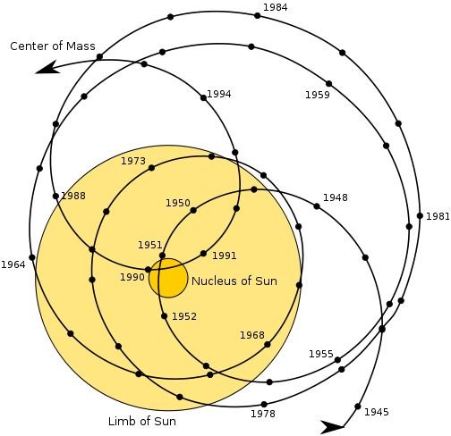
I was wondering, why a pyramid? Because of its relative stability, or is there something else?

pr.probability - Stein's method proof of the Berry-Esséen theorem

The relevant paper is "An estimate of the remainder in a combinatorial central limit theorem" by Erwin Bolthausen. I would like to understand the estimate on page three right before the sentence "where we used independence of $S_{n-1}$ and $X_n$":

$$begin{align}E|f'(S_n) - f'(S_{n-1})|
&le E bigg(frac{|X_n|}{sqrt{n}} big(1 + 2|S_{n-1}| + frac{1}{lambda} int_0^1 1_{[z,z+lambda]} (S_{n-1} + t frac{X_n}{ sqrt{n}}) dtbig)bigg) \
&le frac{C}{sqrt{n}} big(1 + delta(gamma, n-1) / lambdabig)end{align}$$

that is, where $delta(gamma, n-1)/lambda$ shows up, which is the error term in the Berry-Esséen bound.

Here $S_n = sum_{i=1}^n X_i / sqrt{n}$ and $X1, ldots, X_n$ are iid with $E X_i =0$, $E X_i^2 = 1$, and $E|X_i|^3 = gamma$. Furthermore, denote $mathcal{L}_n$ to be the set of all sequences of $n$ random variables satisfying the above assumptions, then

$ delta(lambda, gamma,n) = sup { |E(h_{z,lambda} (S_n)) - Phi(h_{z,lambda})|: z in mathbb{R}, X_1, ldots, X_n in mathcal{L}_n }$

and $h_{z, lambda}(x) = ((1 + (z-x)/lambda) wedge 1) vee 0$ and $delta(gamma, n)$ is a short hand for $delta(0,gamma, n)$, and $h_{z,0}$ is interpreted as $1_{(-infty, z]}$. I am mainly interested in verifying the second inequality, so I don't need to reproduce the definition of $f$ here, but it is related to $h$.

This paper is freely available online through springer. thanks in advance.

ag.algebraic geometry - Can $mathbb{P}^n$ be regarded as an algebraic vector bundle over some algebraic variety?

Stephen Griffeth's argument works over any field. The total space of a vector bundle is never proper (follows by, e.g., valuative criterion for properness). On the other hand, $P^n$ is always proper.

Here is an argument that the total space of a vector bundle is not proper: A fiber of a vector bundle is isomorphic to $A^n$ . Moreover, the fiber considered as a subscheme is a closed subscheme. You can map $(A^1 setminus 0)$ into the fiber by a map like $f(x)=1/x$. This map can't extend over zero, because if it did, then zero would be sent to something in the closure of the fiber. But the fiber is already closed, so zero would be sent to the fiber, contradiction.

---

Edit: Of course, amaanush's answer is a much better answer than mine!

rt.representation theory - closed irreducible subspaces in L²(R)

Taking Fourier transforms, you get the action by multiplication. (Really, $x$ acts by multiplying with $e^{ix}$.) The closed invariant subspaces will thus be of the form ${fin L^2(mathbb{R})colonhat f|_E=0}$ for measurable sets $E$.

But you were asking for closed irreducible subspaces: There aren't any, because the Lebesgue measure has no atoms.

soft question - measure theory for regular cardinals

One answer to your question is to remain within the realm of the continuum, and consider what happens when the Continuum Hypothesis fails. In this case, there are cardinals κ below the continuum c = |R|, and one naturally inquires whether these cardinals behave more like aleph₀, or more like the continuum, with respect to measure and additivity. For example, we may still want to inquire about our favorite measures, but with uncountable cardinals.

The answer is saturated with set-theoretic independence. For example, it is known to be consistent with the axioms of set theory that Lebesgue measure can be better than countably additive! Under Martin's Axiom (MA), when the Continuum Hypothesis fails, then
the union of κ many measure zero sets remains measure zero, for any κ below the continuum. It follows from this that Lebesgue measure is literally ≤κ additive, in the sense that the measure of the union of κ many disjoint sets is the sum of their individual measures (since only countably many of them can have positive measure). This includes the case of uncountable κ, and so goes strictly beyond countable additivity. There are similar results concerning the additivity of the ideal of meager sets.

Indeed, there is a rich subject investigating this called cardinal characteristics of the continuum. I discussed some of the concepts in this MO answer. The point of this subject is to investigate exactly how the dichotomy between countable and continuum plays out in situations when CH fails. Researchers in this area define a number of cardinal invariants, such as:

The bounding number b is the size of the smallest unbounded family of functions from ω to ω. There is no function that bounds every member of the family.

The dominating number d is the size of the smallest dominating family of functions ω to ω. Every function is dominated by a member of the family.

The additivity number for measure is the smallest number of measure zero sets whose union is not measure zero.

The covering number for measure is the smallest number of measure zero sets whose union is all of R.

The uniformity number for measure is the size of the smallest non-measure zero set.

The cofinality number for measure is the smallest size of a family of measure zero sets, such that every measure zero set is contained in one of them.

Each of these numbers is ω₁ under the Continuum Hypothesis, and this expresses the preoccupation with ω that you mention in your question. However, when CH fails, then one cannot prove that any of these numbers is equal to another. Each of them expresses a fundamental characteristic of the continuum, and there are models of set theory distinguishing any two of them (and distinguishing them from ω₁ and the continuum as well).

One can define similar numbers using the ideal of meager sets in place of the ideal of measure zero sets, and the relationships between all these cardinal characteristics are precisely expressed by Cichon's diagram. In particular, no two of them are provably equal, and there are models of set theory exhibiting wide varieties of possible relationships. There are dozens of other cardinal characteristics, whose relationships are the focus of intense study by set theorists working in this area. The main tool for separating these cardinal characteristics is the method of forcing and especially iterated forcing.

---

Another answer to your question is to go well beyond the continuum, and perhaps this is what you are really asking about. The analogue of the theory of cardinal characteristics of the continuum has been carried out for arbitrary cardinals κ, and again, the situation is saturated with independence results, proved by forcing.

For certain types of questions, however, it is interesting to note that there is no intermediate possibility between the countable and large cardinals. For example,
an ultrafilter on a set can be viewed as an ω-complete 2-valued measure on subsets of ω (ω complete = additive for unions of size less than ω = finitely additive). Can one have an Aleph₁ additive ultrafilter on a set? Well, if F is such an ultrafilter, then it must also be Aleph₂ additive, Aleph₃ additive, and so on, for quite a long way, up to the least measurable cardinal. That is, it is just not possible to have a δ-additive ultrafilter, when δ is uncountable, unless it is also additive up to measurable cardinal. Other similar phenomenon surround the question: does every κ additive filter extend to a κ additive ultrafilter on a set? This is true for κ = ω, since this just amounts to being finitely additive, which is what being a filter means. But for uncountable κ, it is equivalent to the assertion that κ is strongly compact, which is very high in the large cardinal hierarchy.

soft question - Too old for advanced mathematics?

With all this unanimous enthusiasm, I can't help but add a cautionary note. I will say, however, that what I'm about to say applies to anyone of any age trying to get a Ph.D. and pursue a career as an academic mathematician.

If you think you want a Ph.D. in mathematics, you should first try your best to talk yourself out of it. It's a little like aspiring to be a pro athlete. Even under the best of circumstances, the chances are too high that you'll end up in a not-very-well-paying job in a not-very-attractive geographic location. Or, if you insist on living in, say, New York, you may end up teaching as an adjunct at several different places.

Someone with your mathematical talents and skills can often find much more rewarding careers elsewhere.

You should pursue the Ph.D. only if you love learning, doing, and teaching mathematics so much that you can't bear the thought of doing anything else, so you're willing to live with the consequences of trying to make a living with one. Or you have an exit strategy should things not work out.

Having said all that, I have a story. When I was at Rice in the mid 80's, a guy in his 40's or 50's came to the math department and told us he really wanted to become a college math teacher. He had always loved math but went into sales(!) and had a very successful career. With enough money stashed away, he wanted to switch to a career in math. To put it mildly, we were really skeptical, mostly because he had the overly cheery outgoing personality of a salesman and therefore was completely unlike anyone else in the math department. It was unthinkable that someone like that could be serious about math. Anyway, we warned him that his goal was probably unrealistic but he was welcome to try taking our undergraduate math curriculum to prepare. Not surprisingly, he found this rather painful, but eventually to our amazement he started to do well in our courses, including all the proofs in analysis. By the end, we told the guy that we thought he really had a shot at getting a Ph.D. and have a modest career as a college math teacher. He thanked us but told us that he had changed his mind. As much as he loved doing the math, it was a solitary struggle and took too much of his time away from his family and friends. In the end, he chose them over a career in math (which of course was a rather shocking choice to us).

So if you really want to do math and can afford to live with the consequences, by all means go for it.

localization - Localizing at the primitive polynomials?

A prime ideal of $S^{-1}R[X]$ is the extension of a unique prime ideal of $R$, so that the morphism $Spec(S^{-1}R[X])to Spec(R)$ is a bijection, and even an homeomorphism. All the extensions of residual fields induced are pure transcendental of transcendence degre $1$.

As an example, if you look at the case $R=mathbb{Z}$, the morphism of schemes you get "puts in family" the extensions of fields $mathbb{F}_phookrightarrowmathbb{F}_p(X)$.

nt.number theory - Local-globalism for similar matrices?

The answer is no. Here is a counter-example
$$left( begin{matrix} 0 & -5 \\ 1 & 0 end{matrix} right) quad mbox{and} quad left( begin{matrix} -1 & -3 \\ 2 & 1 end{matrix} right).$$

Both of these matrices have characteristic polynomial $x^2+5$. For $p neq 2$, $5$, this polynomial has no repeated factors so any matrices with this polynomial are similar. By the same argument, they are similar over $mathbb{Q}$. By brute force computation, they are also similar at $2$ and $5$.

However, they are not similar over $mathbb{Z}$. Consider $mathbb{Z}^2$ as a module for $mathbb{Z}[t]$ where $t$ acts by one of the two matrices above. Both of these matrices square to $-5$, so these are in fact $mathbb{Z}[sqrt{-5}]$-modules. If the matrices were similar, the similarity would give an isomorphism of $mathbb{Z}[sqrt{-5}]$-modules. But these are not isomorphic: the former is free on one generator while the latter is isomorphic to the ideal $langle 2, 1+ sqrt{-5} rangle$.

In general, the way to classify similarity of matrices over $mathbb{Z}$ is the following: If the matrices do not have the same characteristic polynomial over $mathbb{Q}$, they are not similar. If they do, let $f$ be the characteristic polynomial and let $R=mathbb{Z}[t]/f(t)$. Then your matrices give $R$-modules, and the matrices are similar if and only if the $R$-modules are isomorphic. If $R$ is the ring of integers of a number field, then $R$-modules are classified by the ideal class group. In general, they are related to the ideal class group, but there are various correction factors related to how $R$ fails to be the ring of integers of its fraction field (or how it fails to be a domain at all). I don't know the details here.

ac.commutative algebra - If L is a field extension of K, how big is L*/K*?

To add to Franz's nice answer:

Let $mathcal{C}$ be the collection of groups isomorphic to the direct sum of a free abelian group of countable rank with a finite abelian group.
In the case where $L/K$ is a nontrivial finite separable extension of global fields, each of the following groups is in $mathcal{C}$ (and the first two are free):

1) The group of fractional ideals of $K$ (or divisors in the function field case)

2) The group of principal fractional ideals of $K$

3) $K^times$

4) $L^times/K^times$

Proof: The first three can be proved in succession by using infinitude of primes, finiteness of class groups, and the Dirichlet unit theorem.

4) As suggested by t3suji and Franz, Chebotarev shows that the rank is infinite. On the other hand, the following trick shows that $L^times/K^times$ is a subgroup of a group in $mathcal{C}$ (and hence in $mathcal{C}$ itself): Replace $L$ by its Galois closure. Let $sigma_1,ldots,sigma_d$ be the elements of $operatorname{Gal}(L/K)$. Then
$$x mapsto (sigma_1(x)/x,ldots,sigma_d(x)/x)$$
injects $L^times/K^times$ into $L^times times cdots times L^times$,
which is in $mathcal{C}$.

rt.representation theory - Definitions of Hecke algebras

A Hecke algebra describes the most reasonable way to convolve functions or measures on a homogeneous space. Suppose that you have seen the definition of convolution of functions on a vector space, or on a discrete group --- the latter is just the group algebra of the group or some completion. Then how could you reasonably define convolution on a sphere? There is no rotationally invariant way to convolve a general $f$ with a general $g$. However, if $f$ is symmetric around a reference point, say the north pole, then you can define the convolution $f * g$, even if $g$ is arbitrary.

This is the basic idea of the Hecke algebra. The $(n-1)$-sphere is the homogeneous space $SO(n)/SO(n-1)$. A function $g$ on the sphere is a function on left cosets. A function $f$ on the sphere which is symmetric about a reference point is a function on double cosets. If $H subseteq G$ is any pair of compact groups, if $f$ is any continuous function on $Hbackslash G/H$, and if $g$ is any continuous function on $G/H$, then their product in the continuous group algebra is well-defined on $G/H$. The functions on double cosets make an algebra, the Hecke algebra, and the functions on left cosets are a bimodule of the Hecke algebra and the parental group $G$.

It is important for the same reasons that any other kind of convolution is important.

A particular case studied by Hecke Iwahori and others from before quantum algebra was the finite group $GL(n,q)$ and the upper triangular subgroup $B$. This is "the" Hecke algebra; it turns out that it is one algebra with a parameter $q$. Or as Ben says, this generalizes to the Iwahori-Hecke algebra of an algebraic group $G$ with a Borel subgroup $B$.

---

The other place that the Hecke algebra arises is as an interesting deformation of the symmetric group, or rather as a deformation of its group algebra. It has a parameter $q$ and you obtain the symmetric group when $q=1$. As I said, it is also the Hecke algebra of $GL(n,q)/GL(n,q)^+$, where $B = GL(n,q)^+$ is the Borel subgroup of upper-triangular matrices (all of them, not just the unipotent ones). There is a second motivation for the Hecke algebra that I should have mentioned: It immediately gives you a representation of the braid group, and this representation reasonably quickly leads to the Jones polynomial and even the HOMFLY polynomial.

When the Jones and HOMFLY were first discovered, it was simply a remark that the braid group representation was through the same Hecke algebra as the convolutional Hecke algebra for $GL(n,q)/B$ (or equivalently $SL(n,q)/B$). Even so, it's a really good question to confirm this "coincidence", as Arminius asks in the comment. Particularly because it is now a fundamental and useful relation and not a coincidence at all. As Ben explains in his blog post, the first model of the Hecke algebra is important for the categorification of the second model.

The coset space of $GL(n,q)/B$ consists of flags in $mathbb{F}_q^n$, and you can see these more easily using projective geometry. When $n=2$, there is an identity double coset 1 and another double coset $T$. A flag is just a point in $mathbb{P}^1$, and the action of $T$ is to replace the point by the formal sum of the other $q$ points. Thus you immediately get $T^2 = (q-1)T + q.$ When $n=3$, a flag is a point and a line containing it in $mathbb{P}^2$. The two smallest double cosets other than the identity are $T_1$ and $T_2$. $T_1$ acts by moving the point in the line; $T_2$ acts by moving the line containing the point. A little geometry then gives you that $T_1T_2T_1$ and $T_2T_1T_2$ both yield one copy of the largest double coset and nothing else. Thus they are equal; this is the braid relation of the Hecke algebra. When $n ge 3$, the Hecke algebra is given by these same local relations, which must still hold.